So, a while back I had the thought that I wanted to map sw files to an integer, with the property that if the two sw files are structurally equivalent, independent of operator and ket names, they would give the same integer. And if they were different, they would give different integers. I made
an attempt, but didn't get very far. Well, now I have made some progress. BTW, turns out this is quite similar to testing if two
graphs are isomorphic. Our sw files are in general a representation for directed, labelled, weighted graphs. So as a starting point I decided to try finding mappings to integers for the simpler case of undirected, unlabeled (or all the same label, really) and unweighted (all the same coeff of 1) graphs. That is, we needed code to map each node in the graph to an integer, and then combine the results from all nodes with some associative, Abelian function, so that the order we consider the nodes doesn't change the final integer. I decided to use multiplication, but I don't know if there is perhaps an advantage to use some other function.
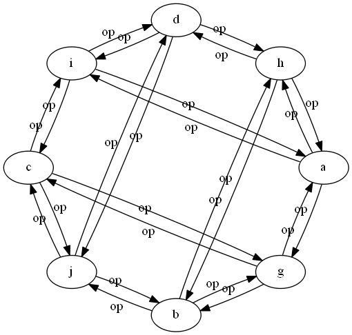
Consider this undirected, unlabeled, unweighted network:
op |A> => |B> + |C> + |G>
op |B> => |A> + |D> + |H>
op |C> => |A> + |D> + |E>
op |D> => |C> + |F> + |B>
op |E> => |C> + |F> + |G>
op |F> => |E> + |D> + |H>
op |G> => |A> + |E> + |H>
op |H> => |G> + |F> + |B>
which has this adjacency matrix:
sa: matrix[op]
[ A ] = [  0  1  1  0  0  0  1  0  ] [ A ]
[ B ]   [  1  0  0  1  0  0  0  1  ] [ B ]
[ C ]   [  1  0  0  1  1  0  0  0  ] [ C ]
[ D ]   [  0  1  1  0  0  1  0  0  ] [ D ]
[ E ]   [  0  0  1  0  0  1  1  0  ] [ E ]
[ F ]   [  0  0  0  1  1  0  0  1  ] [ F ]
[ G ]   [  1  0  0  0  1  0  0  1  ] [ G ]
[ H ]   [  0  1  0  0  0  1  1  0  ] [ H ]
So now what? Well, there are not a lot of options really. About the only one is to consider op^k:
sa: op |A>
|B> + |C> + |G>

sa: op^2 |A>
3|A> + 2|D> + 2|H> + 2|E>

sa: op^3 |A>
7|B> + 7|C> + 7|G> + 6|F>

sa: op^4 |A>
21|A> + 20|D> + 20|H> + 20|E>

sa: op^5 |A>
61|B> + 61|C> + 61|G> + 60|F>
And similarly for say node E:
sa: op |E>
|C> + |F> + |G>

sa: op^2 |E>
2|A> + 2|D> + 3|E> + 2|H>

sa: op^3 |E>
6|B> + 7|C> + 7|G> + 7|F>

sa: op^4 |E>
20|A> + 20|D> + 20|H> + 21|E>

sa: op^5 |E>
60|B> + 61|C> + 61|G> + 61|F>
Now we need some mapping of these superpositions to integers. The simplest is just count the number of kets in each superposition, and sum up the coefficients of the superpositions.
For example:
-- how many kets in op^2 |A>:
sa: how-many op^2 |A>
|number: 4>

-- sum of the coefficients in op^5 |E>:
sa: count-sum op^5 |E>
|number: 243>
Giving this candidate code:
# define our primes:
primes = [2,3,5,7,11,13,17,19,23,29,31,37,41,43,47,53,59,61,67,71]

# define our node to signature function:
# node is a ket, op is a string, k is a positive integer
#
def node_to_signature(node,op,k):
  signature = 1
  r = node
  for n in range(0,2*k+2,2):
    v1 = int(r.count())
    v2 = int(r.count_sum())
    signature *= primes[n]**v1
    signature *= primes[n+1]**v2
    r = r.apply_op(context,op)
  return signature
where:
- r.count() counts the number of kets in the superposition r
- r.count_sum() sums the coefficients in the superposition r
- r.apply_op(context,op) is the backend python for "op |r>"
Multiply the result for each node together, and we get an integer for the entire graph.
For example,
network-1 given above (
code here):
$ ./k_similarity.py

Usage: ./k_similarity.py network.sw k

$ ./k_similarity.py sw-examples/network-1.sw 0
final 0 signature: 1679616

$ ./k_similarity.py sw-examples/network-1.sw 1
final 1 signature: 19179755540281619947585464477539062500000000

$ ./k_similarity.py sw-examples/network-1.sw 2
final 2 signature: 6476350707318135130077117995114645986807357994898007018142410234416950335365537077653915561137590232737115400989220342662084412388620595718383789062500000000

$ ./k_similarity.py sw-examples/network-1.sw 3
final 3 signature: 24915731868195494319495815784319613492832634952662828691337747373649371307162868449881081569598627271299028119958195828952049161143923339977360231242362436120389977749741771679154317963360167622141780171409392307815307137197414891280901439715432140783946679111853342421234802445604704216529913721698446113005853797982997735094149548130522011842820562607650700432722674863502965065307257559822955178526515947974154452386341191890795350397708587635938073745727539062500000000
And yeah, they are quite large integers! So here
is a partial optimization (basically we reverse our list of v's so that the largest v's get applied to the smallest primes):
def node_to_signature(node,op,k):
  signature = 1
  r = node
  v_list = []
  for n in range(0,k+1):
    v1 = int(r.count())
    v2 = int(r.count_sum())
    v_list.append(v1)
    v_list.append(v2)
    r = r.apply_op(context,op)
  v_list.reverse()
  for i,v in enumerate(v_list):
    signature *= primes[i]**v
  return signature
Then apply these to network-1 again:
$ ./k_similarity_v2.py sw-examples/network-1.sw 0
final 0 signature: 1679616
signature log 10: 6.225210003069149
final 0 hash signature: 724e88406ed484a3f47b2c3d522b315261a6b265

$ ./k_similarity_v2.py sw-examples/network-1.sw 1
final 1 signature: 10670244327163201329561600000000
signature log 10: 31.02817436400965
final 1 hash signature: 034f0b554b967c20407ecf3e4373a0c9dde3bdca

$ ./k_similarity_v2.py sw-examples/network-1.sw 2
final 2 signature: 17472747581618922968458849772385108978718944775448150613650671927296000000000000000000000000
signature log 10: 91.24236120296295
final 2 hash signature: d988b544b788f948151bc918dc314cabeecb92a4

$ ./k_similarity_v2.py sw-examples/network-1.sw 3
final 3 signature: 28908255527868889825790269007077519960587554847149293166812397097145900954989327674871077402331703366281633882780425402405190443720178454553217647654140379136000000000000000000000000000000000000000000000000000000000000000000000000
signature log 10: 229.461021884909
final 3 hash signature: 39d6e5cdc2300c06801865ddf558c3bfbdf03e16
Which is a big improvement in signature integer size. There are probably other optimizations that could be made, but I'm happy enough with this.
Now we are ready to throw it at some networks:
network 2:
op |A> => |B> + |E> + |G>
op |B> => |A> + |E> + |C>
op |C> => |B> + |F> + |D>
op |D> => |C> + |F> + |H>
op |E> => |A> + |B> + |G>
op |F> => |C> + |D> + |H>
op |G> => |A> + |E> + |H>
op |H> => |G> + |F> + |D>

final 0 signature: 1679616
signature log 10: 6.225210003069149
final 0 hash signature: 724e88406ed484a3f47b2c3d522b315261a6b265

final 1 signature: 10670244327163201329561600000000
signature log 10: 31.02817436400965
final 1 hash signature: 034f0b554b967c20407ecf3e4373a0c9dde3bdca

final 2 signature: 752144490249374505343739906132775290761509353163124189431799265916843196416000000000000000000000000
signature log 10: 98.87630127847756
final 2 hash signature: c3a6b9f345a2b76c165fb3c997542110f9bd3051

final 3 signature: 1780207704063630331903810305642872528743446816219521629215268406907491725204135233958145047922812087077527584194258689629049352975220203052830112622815055508579908457300235611841260158976000000000000000000000000000000000000000000000000000000000000000000000000
signature log 10: 258.25047067616634
final 3 hash signature: 50806a21d5f34dbb85d098f4ecabdfe9c6e1052d
network 3:
op |a> => |g> + |h> + |i>
op |b> => |g> + |h> + |j>
op |c> => |g> + |i> + |j>
op |d> => |h> + |i> + |j>
op |g> => |a> + |b> + |c>
op |h> => |a> + |b> + |d>
op |i> => |a> + |c> + |d>
op |j> => |b> + |c> + |d>

final 0 signature: 1679616
signature log 10: 6.225210003069149
final 0 hash signature: 724e88406ed484a3f47b2c3d522b315261a6b265

final 1 signature: 10670244327163201329561600000000
signature log 10: 31.02817436400965
final 1 hash signature: 034f0b554b967c20407ecf3e4373a0c9dde3bdca

final 2 signature: 17472747581618922968458849772385108978718944775448150613650671927296000000000000000000000000
signature log 10: 91.24236120296295
final 2 hash signature: d988b544b788f948151bc918dc314cabeecb92a4

final 3 signature: 28908255527868889825790269007077519960587554847149293166812397097145900954989327674871077402331703366281633882780425402405190443720178454553217647654140379136000000000000000000000000000000000000000000000000000000000000000000000000
signature log 10: 229.461021884909
final 3 hash signature: 39d6e5cdc2300c06801865ddf558c3bfbdf03e16
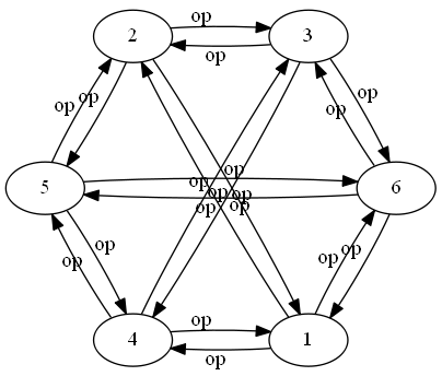
network-5:
op |1> => |6> + |4> + |2>
op |2> => |1> + |5> + |3>
op |3> => |2> + |6> + |4>
op |4> => |3> + |1> + |5>
op |5> => |6> + |4> + |2>
op |6> => |1> + |3> + |5>

final 0 signature: 46656
signature log 10: 4.668907502301861
final 0 hash signature: f89664dd10bc575affd2df12323f9fa1386bec50

final 1 signature: 186694177220038656000000
signature log 10: 23.27113077300724
final 1 hash signature: 43361818928df1e25cf2d42eaf826b9b79e535ad

final 2 signature: 370717744295392913280583372681517644759594696704000000000000000000
signature log 10: 65.56904337390424
final 2 hash signature: 5acae2f217c04b462739d64df04d8cfddd030ebf

final 3 signature: 145361918192683278731003716769548827497223900554742033134393018706053787797668034552637435114664336624164274176000000000000000000000000000000000000000000000000000000
signature log 10: 164.16245064527826
final 3 hash signature: d12513fc0a3ec0439083640a6b366d7c478d8c75
And we note that network-1 and network-3 agree for k in {0,1,2,3}, and network-2 only agrees for k in {0,1}. Indeed, this is a pattern I saw with all the networks I tested. If they were isomorphic they agreed for all tested k (indeed, my algo would be broken if isomorphic graphs have a k where they differ in signature), and if they have the same number of vertices and edges per vertex, but are not isomorphic, they agree for k in {0,1}, but differ at k = 2. Note that network-5 has only 6 nodes, instead of 8, so it doesn't even agree with network-1, network-2 and network-3 at k = 0.
Now for some comments:
1) isomorphic graphs should produce the same signature for all k. If not, then my algo is broken!
2) what is the smallest k such that we can be sure graphs are not isomorphic? I don't know. In all the examples I tested k = 2 was sufficient. But presumably there can be collisions where non-isomorphic graphs produce the same signature for some k. So that means we can only prove graphs are not isomorphic if we have a k where they differ, but we can only be probably sure they are isomorphic if we haven't found a k where they differ.
3) if two graphs differ at k, then presumably, baring some weird collision, they will also differ for all larger k.
4) k = 0 is directly related to node count.
5) k = 1 is directly related to the number of edges connected to each vertex
6) just because we are probably sure two graphs are isomorphic doesn't help at all in finding that isomorphism.
7) there is a matrix version of my algo. Though I'm not sure when my algo is cheaper, and when the matrix version is cheaper. Consider k = 2. This corresponds to op^2 |some node>, and to this matrix:
sa: merged-matrix[op,op]
[ A ] = [  3  0  0  2  2  0  0  2  ] [ A ]
[ B ]   [  0  3  2  0  0  2  2  0  ] [ B ]
[ C ]   [  0  2  3  0  0  2  2  0  ] [ C ]
[ D ]   [  2  0  0  3  2  0  0  2  ] [ D ]
[ E ]   [  2  0  0  2  3  0  0  2  ] [ E ]
[ F ]   [  0  2  2  0  0  3  2  0  ] [ F ]
[ G ]   [  0  2  2  0  0  2  3  0  ] [ G ]
[ H ]   [  2  0  0  2  2  0  0  3  ] [ H ]
Now consider the columns separately. v1 of the first column is the number of elements with coeff > 0. ie, in this case 4. v2 is the sum of the elements in the column. ie, in this case 9. Then our integer for this column is (p1^v1)*(p2^v2) for some primes p1 and p2. Do similarly for the other columns, multiply the results together, and then you have your graph signature integer. How to do that for other k should be obvious. Actually, my algo is slightly different from this. It takes all values of {0,1,...,k} into account, not just the given k. See the code above, to clarify!
8) there are probably other ways to map op^k |some node> superpositions to integers.
9) there are probably optimizations to my method.
10) it can be a little bit of work converting diagrams to BKO notation
11) it shouldn't be hard to convert this code to handle more general sw files. I'll probably try that tomorrow.
12) recall we noted
some similarities between category theory and BKO. If we show that two sw files are almost certainly isomorphic, this implies there exists a functor mapping one sw file to the other.
13) we can use our project to easily find k-cycles in networks. No claims about efficiency though! Simply enough, node |x> has a k-cycle if |x> is a member of the op^k |x> superposition.
Now in BKO:
sa: load network-1.sw
sa: has-3-cycle |*> #=> is-mbr(|_self>,op^3 |_self>)
sa: has-4-cycle |*> #=> is-mbr(|_self>,op^4 |_self>)
sa: has-5-cycle |*> #=> is-mbr(|_self>,op^5 |_self>)
sa: has-6-cycle |*> #=> is-mbr(|_self>,op^6 |_self>)
sa: has-7-cycle |*> #=> is-mbr(|_self>,op^7 |_self>)
sa: has-8-cycle |*> #=> is-mbr(|_self>,op^8 |_self>)
sa: has-9-cycle |*> #=> is-mbr(|_self>,op^9 |_self>)
sa: has-10-cycle |*> #=> is-mbr(|_self>,op^10 |_self>)

sa: table[node,has-3-cycle,has-4-cycle,has-5-cycle,has-6-cycle,has-7-cycle,has-8-cycle,has-9-cycle,has-10-cycle] rel-kets[op]
+------+-------------+-------------+-------------+-------------+-------------+-------------+-------------+--------------+
| node | has-3-cycle | has-4-cycle | has-5-cycle | has-6-cycle | has-7-cycle | has-8-cycle | has-9-cycle | has-10-cycle |
+------+-------------+-------------+-------------+-------------+-------------+-------------+-------------+--------------+
| A    | no          | yes         | no          | yes         | no          | yes         | no          | yes          |
| B    | no          | yes         | no          | yes         | no          | yes         | no          | yes          |
| C    | no          | yes         | no          | yes         | no          | yes         | no          | yes          |
| D    | no          | yes         | no          | yes         | no          | yes         | no          | yes          |
| E    | no          | yes         | no          | yes         | no          | yes         | no          | yes          |
| F    | no          | yes         | no          | yes         | no          | yes         | no          | yes          |
| G    | no          | yes         | no          | yes         | no          | yes         | no          | yes          |
| H    | no          | yes         | no          | yes         | no          | yes         | no          | yes          |
+------+-------------+-------------+-------------+-------------+-------------+-------------+-------------+--------------+

sa: reset
sa: load network-2.sw
sa: load has-k-cycle.sw
sa: table[node,has-3-cycle,has-4-cycle,has-5-cycle,has-6-cycle,has-7-cycle,has-8-cycle,has-9-cycle,has-10-cycle] rel-kets[op]
+------+-------------+-------------+-------------+-------------+-------------+-------------+-------------+--------------+
| node | has-3-cycle | has-4-cycle | has-5-cycle | has-6-cycle | has-7-cycle | has-8-cycle | has-9-cycle | has-10-cycle |
+------+-------------+-------------+-------------+-------------+-------------+-------------+-------------+--------------+
| A    | yes         | yes         | yes         | yes         | yes         | yes         | yes         | yes          |
| B    | yes         | yes         | yes         | yes         | yes         | yes         | yes         | yes          |
| C    | yes         | yes         | yes         | yes         | yes         | yes         | yes         | yes          |
| D    | yes         | yes         | yes         | yes         | yes         | yes         | yes         | yes          |
| E    | yes         | yes         | yes         | yes         | yes         | yes         | yes         | yes          |
| F    | yes         | yes         | yes         | yes         | yes         | yes         | yes         | yes          |
| G    | yes         | yes         | yes         | yes         | yes         | yes         | yes         | yes          |
| H    | yes         | yes         | yes         | yes         | yes         | yes         | yes         | yes          |
+------+-------------+-------------+-------------+-------------+-------------+-------------+-------------+--------------+

sa: reset
sa: load network-5.sw
sa: load has-k-cycle.sw
sa: table[node,has-3-cycle,has-4-cycle,has-5-cycle,has-6-cycle,has-7-cycle,has-8-cycle,has-9-cycle,has-10-cycle] rel-kets[op]
+------+-------------+-------------+-------------+-------------+-------------+-------------+-------------+--------------+
| node | has-3-cycle | has-4-cycle | has-5-cycle | has-6-cycle | has-7-cycle | has-8-cycle | has-9-cycle | has-10-cycle |
+------+-------------+-------------+-------------+-------------+-------------+-------------+-------------+--------------+
| 1    | no          | yes         | no          | yes         | no          | yes         | no          | yes          |
| 2    | no          | yes         | no          | yes         | no          | yes         | no          | yes          |
| 3    | no          | yes         | no          | yes         | no          | yes         | no          | yes          |
| 4    | no          | yes         | no          | yes         | no          | yes         | no          | yes          |
| 5    | no          | yes         | no          | yes         | no          | yes         | no          | yes          |
| 6    | no          | yes         | no          | yes         | no          | yes         | no          | yes          |
+------+-------------+-------------+-------------+-------------+-------------+-------------+-------------+--------------+

sa: reset
sa: load network-7.sw
sa: load has-k-cycle.sw
sa: table[node,has-3-cycle,has-4-cycle,has-5-cycle,has-6-cycle,has-7-cycle,has-8-cycle,has-9-cycle,has-10-cycle] rel-kets[op]
+------+-------------+-------------+-------------+-------------+-------------+-------------+-------------+--------------+
| node | has-3-cycle | has-4-cycle | has-5-cycle | has-6-cycle | has-7-cycle | has-8-cycle | has-9-cycle | has-10-cycle |
+------+-------------+-------------+-------------+-------------+-------------+-------------+-------------+--------------+
| a    | no          | yes         | yes         | yes         | yes         | yes         | yes         | yes          |
| b    | no          | yes         | yes         | yes         | yes         | yes         | yes         | yes          |
| c    | no          | yes         | yes         | yes         | yes         | yes         | yes         | yes          |
| d    | no          | yes         | yes         | yes         | yes         | yes         | yes         | yes          |
| e    | no          | yes         | yes         | yes         | yes         | yes         | yes         | yes          |
| f    | no          | yes         | yes         | yes         | yes         | yes         | yes         | yes          |
| g    | no          | yes         | yes         | yes         | yes         | yes         | yes         | yes          |
| h    | no          | yes         | yes         | yes         | yes         | yes         | yes         | yes          |
| i    | no          | yes         | yes         | yes         | yes         | yes         | yes         | yes          |
| j    | no          | yes         | yes         | yes         | yes         | yes         | yes         | yes          |
+------+-------------+-------------+-------------+-------------+-------------+-------------+-------------+--------------+

sa: reset
sa: load network-11.sw
sa: load has-k-cycle.sw
sa: table[node,has-3-cycle,has-4-cycle,has-5-cycle,has-6-cycle,has-7-cycle,has-8-cycle,has-9-cycle,has-10-cycle] rel-kets[op]
+------+-------------+-------------+-------------+-------------+-------------+-------------+-------------+--------------+
| node | has-3-cycle | has-4-cycle | has-5-cycle | has-6-cycle | has-7-cycle | has-8-cycle | has-9-cycle | has-10-cycle |
+------+-------------+-------------+-------------+-------------+-------------+-------------+-------------+--------------+
| 1    | yes         | yes         | yes         | yes         | yes         | yes         | yes         | yes          |
| 2    | yes         | yes         | yes         | yes         | yes         | yes         | yes         | yes          |
| 3    | yes         | yes         | yes         | yes         | yes         | yes         | yes         | yes          |
| 4    | no          | yes         | yes         | yes         | yes         | yes         | yes         | yes          |
| 5    | no          | yes         | yes         | yes         | yes         | yes         | yes         | yes          |
| 6    | yes         | yes         | yes         | yes         | yes         | yes         | yes         | yes          |
+------+-------------+-------------+-------------+-------------+-------------+-------------+-------------+--------------+
So that is all kind of pretty. But my hunch is that mapping node cycle counts to signature integers is more expensive than my method. Note that 2-cycles are boring. In an undirected graph, all nodes have 2-cycles.
14) when can we expect collisions? Consider network A and network B. For some node, and k, they have superpositions r1 and r2 respectively. We will have a collision if r1.count() == r2.count() and r1.count_sum() == r2.count_sum() yet r1 and r2 are not equal. Presumably, this will not persist for other values of k. I don't know for sure though!
15) it would be nice to have examples of non-isomorphic graphs yet they agree for at least k = 2. All the non-iso examples I tested had different k = 2 signatures.
16) let's find k = 2 signatures for all our networks:
network 1:
final 2 hash signature: d988b544b788f948151bc918dc314cabeecb92a4

network 2:
final 2 hash signature: c3a6b9f345a2b76c165fb3c997542110f9bd3051

network 3:
final 2 hash signature: d988b544b788f948151bc918dc314cabeecb92a4

network 4:
final 2 hash signature: d988b544b788f948151bc918dc314cabeecb92a4

network 5:
final 2 hash signature: 5acae2f217c04b462739d64df04d8cfddd030ebf

network 6:
final 2 hash signature: 5acae2f217c04b462739d64df04d8cfddd030ebf

network 7:
final 2 hash signature: 6853d10f768067b82119e5fe99d6a8969d569477

network 8:
final 2 hash signature: caef2fb67b25a750cefdc11d05219695db55326b

network 9:
final 2 hash signature: 6ca9d1097590e86b4af0c59e746e10d5caf803fb

network 10:
final 2 hash signature: 6ca9d1097590e86b4af0c59e746e10d5caf803fb

network 11:
final 2 hash signature: 2050930de8495fea7b75b0b1dadc51462dbead44

network 12:
final 2 hash signature: 36256c6db2fe1e6c9a4f937e8d2f535b747a4e15

network 13:
final 2 hash signature: cb3f6e656e8ecd1818a9ae08f51e6cd3437743f1

network 14:
final 2 hash signature: 08786357aa7d977507caaced7f292c95946f11b8

network 16:
final 2 hash signature: d988b544b788f948151bc918dc314cabeecb92a4

network 17:
final 2 hash signature: 5acae2f217c04b462739d64df04d8cfddd030ebf

network 18:
final 2 hash signature: 5acae2f217c04b462739d64df04d8cfddd030ebf

network 20:
final 2 hash signature: 4c5182ec30e09c9b09f3980a3998381ea3404035
Resulting in this classification:
{1,3,4,16}
{2}
{5,6,17,18}
{7}
{8}
{9,10}
{11}
{12}
{13}
{14}
{20}
17) it would be nice to test this code on larger networks, say something with 50 nodes instead of just 8.
Update: wrote some code to do the classification for me:
$ ./k_classifier.py

Usage: ./k_classifier.py k network-1.sw [network-2.sw network-3.sw ...]

$ ./k_classifier.py 0 sw-examples/network-*.sw
the k = 0 network classes:
----------------------------
724e88406ed484a3f47b2c3d522b315261a6b265: network-1, network-16, network-2, network-20, network-21, network-22, network-3, network-4
f60f6fcc93727388d031d7eada90c959c0813ca0: network-10, network-7, network-8, network-9
f89664dd10bc575affd2df12323f9fa1386bec50: network-11, network-12, network-17, network-18, network-23, network-24, network-5, network-6
cd0bcbc7f5b13e9aa1cae35d665739eb964f2084: network-13, network-14
----------------------------

the k = 1 network classes:
----------------------------
034f0b554b967c20407ecf3e4373a0c9dde3bdca: network-1, network-16, network-2, network-20, network-3, network-4
5328d58c5e05fa27d819aa197355238f2364456b: network-10, network-7, network-8, network-9
7ccf6241d30bfc88bd65e22dbdfe7488c67ca41d: network-11, network-12, network-23, network-24
cb38319a6c5110625a9085c7c110b213ea82621c: network-13, network-14
43361818928df1e25cf2d42eaf826b9b79e535ad: network-17, network-18, network-5, network-6
49063e880677302c51a3d93774ed58c328d909a5: network-21, network-22
----------------------------

the k = 2 network classes:
----------------------------
d988b544b788f948151bc918dc314cabeecb92a4: network-1, network-16, network-3, network-4
6ca9d1097590e86b4af0c59e746e10d5caf803fb: network-10, network-9
2050930de8495fea7b75b0b1dadc51462dbead44: network-11, network-23
36256c6db2fe1e6c9a4f937e8d2f535b747a4e15: network-12, network-24
cb3f6e656e8ecd1818a9ae08f51e6cd3437743f1: network-13
08786357aa7d977507caaced7f292c95946f11b8: network-14
5acae2f217c04b462739d64df04d8cfddd030ebf: network-17, network-18, network-5, network-6
c3a6b9f345a2b76c165fb3c997542110f9bd3051: network-2
4c5182ec30e09c9b09f3980a3998381ea3404035: network-20
863a20a85da3519434ef062f6f6ce3d7ef205582: network-21, network-22
6853d10f768067b82119e5fe99d6a8969d569477: network-7
caef2fb67b25a750cefdc11d05219695db55326b: network-8
----------------------------

the k = 3 network classes:
----------------------------
39d6e5cdc2300c06801865ddf558c3bfbdf03e16: network-1, network-16, network-3, network-4
c5d102de3b83458cd8132e3f2548eba762c21ab1: network-10, network-9
a94c9bed956e401ce7b6a123a9b346fb0ecf7cb9: network-11, network-23
434be5de95678a144fcc201ccdd5de2ccb1e9bd2: network-12, network-24
f946ed753556eeb940fff9e1cc917c0864ca8d61: network-13
10e26cdc3fc270f2a77cff5744074163d142ad47: network-14
d12513fc0a3ec0439083640a6b366d7c478d8c75: network-17, network-18, network-5, network-6
50806a21d5f34dbb85d098f4ecabdfe9c6e1052d: network-2
7a8f9bf7116d347b36de0394cab2c0ef28056fd4: network-20
2ee33d74438b11c8f8d77c46795f747ae42350a7: network-21
a12436ce936de85984532aa6e6106de076d4f1e3: network-22
b49f21325227d1dbd242c8f2e24f7bb9cbef40d8: network-7
b8652c9f1b37544e3c121ca18bb43b2eba68ce7f: network-8
----------------------------

the k = 4 network classes:
----------------------------
19a289b17734656ea7b096a10ebbcf128aed91a7: network-1, network-16, network-3, network-4
121e741ac6e8409ffef76b7622cfedbe00a1caab: network-10, network-9
7fb17280e48ed0db64ee57da273e7f0ddf142e27: network-11, network-23
7da034f87ed041af85945f8d4dd7911fffe8cf6c: network-12, network-24
75b0417b9b995e076c328bef991ae9b55cd6650e: network-13
ded50780072d4c51bd2441e75a01c0389d713402: network-14
3ada223550705dbc27fabbc19cb5e03983330344: network-17, network-18, network-5, network-6
631eae539d43d5402da693888f0231022bd12ca8: network-2
1988a1e18c7e0053814483f7d7cbef04da8a1d07: network-20
f37d01cb4642923151e0ada1b044a83fe5a02fa4: network-21
148619ef3a39ce65b167cadf71180234e45f920c: network-22
21b00bfd65d6608cef200d486357dbd1bceeacd3: network-7
9fc685480e63c1551a325b27b1992e5a14d1ede8: network-8
----------------------------
BTW, in
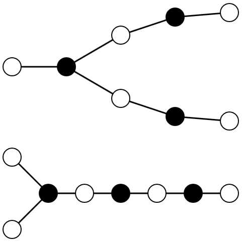
reading around, I finally found an example where they are not isomorphic, but agree at k = 2, but disagree at k = 3 and k = 4. These graphs are given as an example of two graphs which have the same degree sequence, yet are not isomorphic. Since my code can distinguish them at k = 3, that means my code is doing something different than degree sequences. These graphs BTW, are
network-21 and
network-22. See the network classes just above. Here are their signatures:
network 21:
op |a> => |b>
op |b> => |a> + |c> + |f>
op |c> => |b> + |d>
op |d> => |c> + |e>
op |e> => |d>
op |f> => |b> + |g>
op |g> => |f> + |h>
op |h> => |g>

$ ./k_similarity_v2.py sw-examples/network-21.sw k
final 0 hash signature: 724e88406ed484a3f47b2c3d522b315261a6b265
final 1 hash signature: 49063e880677302c51a3d93774ed58c328d909a5
final 2 hash signature: 863a20a85da3519434ef062f6f6ce3d7ef205582
final 3 hash signature: 2ee33d74438b11c8f8d77c46795f747ae42350a7
final 4 hash signature: f37d01cb4642923151e0ada1b044a83fe5a02fa4

network 22:
op |a> => |b>
op |b> => |a> + |c> + |d>
op |c> => |b>
op |d> => |b> + |e>
op |e> => |d> + |f>
op |f> => |e> + |g>
op |g> => |f> + |h>
op |h> => |g>

final 0 hash signature: 724e88406ed484a3f47b2c3d522b315261a6b265
final 1 hash signature: 49063e880677302c51a3d93774ed58c328d909a5
final 2 hash signature: 863a20a85da3519434ef062f6f6ce3d7ef205582
final 3 hash signature: a12436ce936de85984532aa6e6106de076d4f1e3
final 4 hash signature: 148619ef3a39ce65b167cadf71180234e45f920c
Here is what they look like (
borrowed from wikipedia):
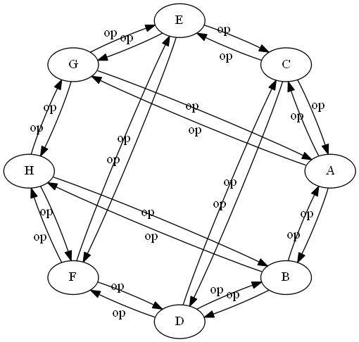
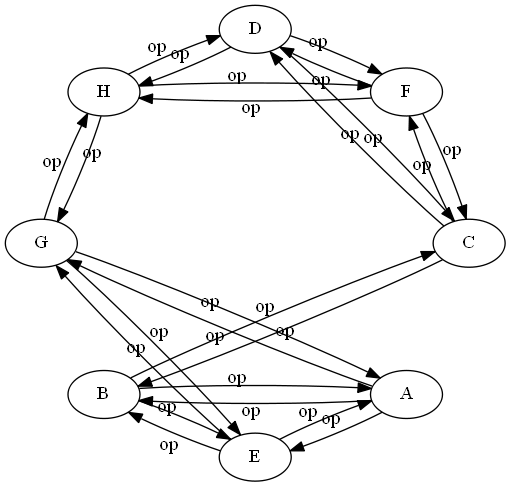
And we can make pretty pictures of our other graphs, using
sw2dot-v2.py and
graphviz:
network 1:
network 2:
network 3:
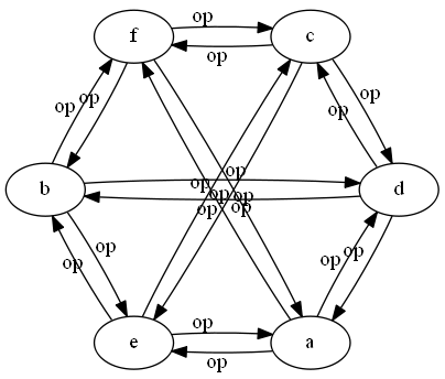
network 5:
network 6:
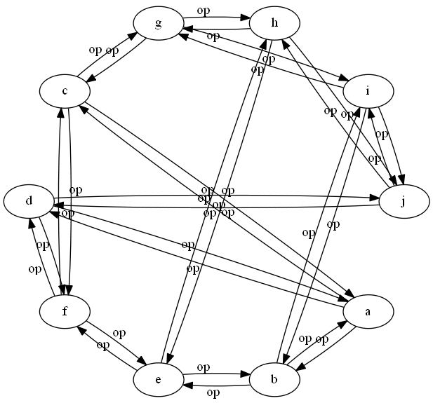
network 7:
network 8:
And so on for our other networks.
Heh. Just occurred to me we can do second order network similarity. Though I'm not exactly sure why you would want to, other than to note it as a theoretical possibility. Perhaps it might be useful if you have a very large number of networks, and you are having trouble visually separating the results from different k's.
Consider this from above (and the rest):
the k = 0 network classes:
----------------------------
network-1, network-16, network-2, network-20, network-21, network-22, network-3, network-4
network-10, network-7, network-8, network-9
network-11, network-12, network-17, network-18, network-23, network-24, network-5, network-6
network-13, network-14
----------------------------
We can massage these into their own sw/networks:
2nd-order-k0-network:
op |1> => |network-1> + |network-16> + |network-2> + |network-20> + |network-21> + |network-22> + |network-3> + |network-4>
op |2> => |network-10> + |network-7> + |network-8> + |network-9>
op |3> => |network-11> + |network-12> + |network-17> + |network-18> + |network-23> + |network-24> + |network-5> + |network-6>
op |4> => |network-13> + |network-14>


2nd-order-k1-network:
op |1> => |network-1> + |network-16> + |network-2> + |network-20> + |network-3> + |network-4>
op |2> => |network-10> + |network-7> + |network-8> + |network-9>
op |3> => |network-11> + |network-12> + |network-23> + |network-24>
op |4> => |network-13> + |network-14>
op |5> => |network-17> + |network-18> + |network-5> + |network-6>
op |6> => |network-21> + |network-22>


2nd-order-k2-network:
op |1> => |network-1> + |network-16> + |network-3> + |network-4>
op |2> => |network-10> + |network-9>
op |3> => |network-11> + |network-23>
op |4> => |network-12> + |network-24>
op |5> => |network-13>
op |6> => |network-14>
op |7> => |network-17> + |network-18> + |network-5> + |network-6>
op |8> => |network-2>
op |9> => |network-20>
op |10> => |network-21> + |network-22>
op |11> => |network-7>
op |12> => |network-8>


2nd-order-k3-network:
op |1> => |network-1> + |network-16> + |network-3> + |network-4>
op |2> => |network-10> + |network-9>
op |3> => |network-11> + |network-23>
op |4> => |network-12> + |network-24>
op |5> => |network-13>
op |6> => |network-14>
op |7> => |network-17> + |network-18> + |network-5> + |network-6>
op |8> => |network-2>
op |9> => |network-20>
op |10> => |network-21>
op |11> => |network-22>
op |12> => |network-7>
op |13> => |network-8>


2nd-order-k4-network:
op |1> => |network-1> + |network-16> + |network-3> + |network-4>
op |2> => |network-10> + |network-9>
op |3> => |network-11> + |network-23>
op |4> => |network-12> + |network-24>
op |5> => |network-13>
op |6> => |network-14>
op |7> => |network-17> + |network-18> + |network-5> + |network-6>
op |8> => |network-2>
op |9> => |network-20>
op |10> => |network-21>
op |11> => |network-22>
op |12> => |network-7>
op |13> => |network-8>

2nd-order-k5-network:
op |1> => |network-1> + |network-16> + |network-3> + |network-4>
op |2> => |network-10> + |network-9>
op |3> => |network-11> + |network-23>
op |4> => |network-12> + |network-24>
op |5> => |network-13>
op |6> => |network-14>
op |7> => |network-17> + |network-18> + |network-5> + |network-6>
op |8> => |network-2>
op |9> => |network-20>
op |10> => |network-21>
op |11> => |network-22>
op |12> => |network-7>
op |13> => |network-8>
Now apply the classifier to these 2nd order networks:
$ ./k_classifier.py 0 sw-examples/2nd-order-k*.sw
the k = 0 network classes:
----------------------------
64c84e952453cd25d3097c7cfb8ba8178a0d109f: 2nd-order-k0-network
f89664dd10bc575affd2df12323f9fa1386bec50: 2nd-order-k1-network
ed7eef2a04f04526c88f43d3f111242289ec7a02: 2nd-order-k2-network
ef27f9e773963f00db02e38621d9f7bfa59e70be: 2nd-order-k3-network, 2nd-order-k4-network, 2nd-order-k5-network
----------------------------
Noting that there is no need to consider k > 0, you will get the same result for all k. This result also shows, if it wasn't already obvious, that we need to consider k = 3 before our classes stabilize. I don't know why you would want to, but no reason you couldn't consider 3rd order, and higher. Maybe like you have categories, categories of categories, and so on. NB: we kind of cheated! Our 2nd order networks are directed, not undirected.
Finally, lets loop back to our knowledge representation, and display the class results in BKO notation:
$ ./k_classifier.py 1 sw-examples/network-*.sw

the k = 1 network classes:
----------------------------
034f0b554b967c20407ecf3e4373a0c9dde3bdca: network-1, network-16, network-2, network-20, network-3, network-4
5328d58c5e05fa27d819aa197355238f2364456b: network-10, network-7, network-8, network-9
7ccf6241d30bfc88bd65e22dbdfe7488c67ca41d: network-11, network-12, network-23, network-24
cb38319a6c5110625a9085c7c110b213ea82621c: network-13, network-14
43361818928df1e25cf2d42eaf826b9b79e535ad: network-17, network-18, network-5, network-6
49063e880677302c51a3d93774ed58c328d909a5: network-21, network-22
----------------------------

2nd-order-k1-network:
class |1> => |network-1> + |network-16> + |network-2> + |network-20> + |network-3> + |network-4>
class |2> => |network-10> + |network-7> + |network-8> + |network-9>
class |3> => |network-11> + |network-12> + |network-23> + |network-24>
class |4> => |network-13> + |network-14>
class |5> => |network-17> + |network-18> + |network-5> + |network-6>
class |6> => |network-21> + |network-22>

hash |1> => |034f0b554b967c20407ecf3e4373a0c9dde3bdca>
hash |2> => |5328d58c5e05fa27d819aa197355238f2364456b>
hash |3> => |7ccf6241d30bfc88bd65e22dbdfe7488c67ca41d>
hash |4> => |cb38319a6c5110625a9085c7c110b213ea82621c>
hash |5> => |43361818928df1e25cf2d42eaf826b9b79e535ad>
hash |6> => |49063e880677302c51a3d93774ed58c328d909a5>
Whew! That's it I think. Next I will have to look into mapping more general sw files to classes. Though I think we will run into some trouble for superpositions that have coefficients not equal to 1.


